
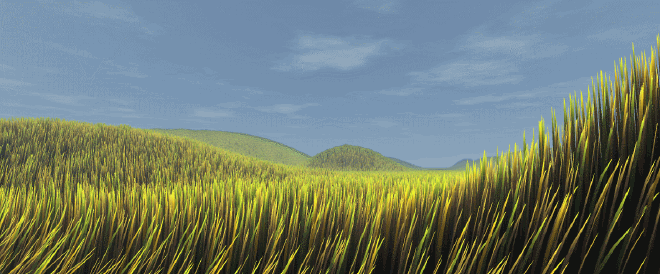
In 2018 after finishing my master thesis and before starting with my PhD I was curious to learn Golang. For me learning a new programming language is most interesting when combining it with a project. During that time I stumbled upon a video which showed a vast scene completely covered in grass. The video was a showcase of Eddie Lee’s master thesis about real-time rendering of grass. The meditative music as well as the way the grass was waving in the wind fascinated me and so I made this Real-Time Grass Rendering demo my Golang project.
To collect further information I checked out Eddie Lee’s website and found a link to his thesis — which seems to be unavailable by now — which I used as basis for my implementation.
The general structure of the demo consists of:
- a seemingly infinite landscape modelled by a seamless heightmap
- each grass blade rendered using a billboard approach
- grass being affected by wind
- using randomization to add more realism
- background displayed using a skybox approach
- some additional post-processing effects
By simply rendering each grass blade individually, the GPU would at some point come to a halt. Furthermore its impossible to render an infinite landscape. We will look at certain aspects of the real-time grass demo and give hints on how it could be implemented. After that I’ll highlight some areas of my implementation that could be further improved. Lastly a link to my Github repository is provided where you can look at the my implementation.
1 The terrain#
The naïve way to visualize a terrain is to create a uniform grid and offset the grid cell points by the height of the terrain to generate a 3D landscape. To make the landscape smooth enough the resolution of this grad has to be high enough. For big landscapes with many hills and valleys this resolution can quickly results in millions of cells. Not all graphic cards support rendering quads so its more reasonable to split a cell into two triangles. Therefore we might have to draw more than two million triangles and this is only the landscape without any grass.
We’ll go into detail how the data structure of the terrain looks like and then introduce how we can save more memory of the seemingly infinite terrain.
1.1 Terrain structure#
Not all areas of the landscape have hills, some areas might even be flat. We might be tempted to use a non-uniform grid and use less triangles where the terrain is almost flat and more triangles in complex areas (e.g. where we have curved shapes). While having potentially less triangles we have an added complexity as we either use some form of Quadtree and have to switch between levels or we use a non-uniform grid where we have to remember the vertex positions. While we could do that it adds unnecessary complexity when collecting the geometry for our render pass.

Another idea that we might have is that we have a limited field of view. What’s the last time that you’ve seen what is behind you without using a mirror or a selfie camera? Thus we can save on processing power by not taking into account geometry that is outside our field of view. In order to do so we split our landscape into chunks — illustrated by the blue quad in the figure above. These chunks shouldn’t be too small since we need to check for each chunk — potentially each frame — if it is in our field of vision or not. However this is no problem as each patch consists of a portion of our tiles of the uniform grid that we have mentioned before. In red we have simply illustrated that each cell or tile consists of two triangles.
| |
We encode each tile as can be seen in the code snippet above. The slope of both triangles that make up the tile can be specified using one normal per triangle. As you can see the normals are a vec4, we actually encode A,B,C,D of the plane equation Ax+By+Cz+D=0 where ABC is the plane normal xyz is any point that lies on the plane and D is the distance of the plane from the origin. We can calculate the two plane normals by getting the positions of the four vertices that make up our tile. For each of them we sample the height map at their position. Next for each of the two triangles we can then first calculate the normals
$$ \mathbf{n}_1 = \frac{\mathbf{v}_2 - \mathbf{v}_1}{|\mathbf{v}_2 - \mathbf{v}_1|} \times \frac{\mathbf{v}_3 - \mathbf{v}_1}{|\mathbf{v}_3 - \mathbf{v}_1|} $$ $$ \mathbf{n}_2 = \frac{\mathbf{v}_3 - \mathbf{v}_4}{|\mathbf{v}_3 - \mathbf{v}_4|} \times \frac{\mathbf{v}_2 - \mathbf{v}_4}{|\mathbf{v}_2 - \mathbf{v}_4|} $$

by calculating the cross product between the normalized vectors between the points of the triangle. The order of the cross product is important as the normals might otherwise point down. Finally we have to calculate the distance of the triangle from the origin. The distance D can be calculate by
$$ D = -Ax -By -Cz $$
where \(A, B, C\) are the components of the triangle normal \( \mathbf{n} \) and \(x, y, z\) are the components of a point that lies on the plane. As the point is arbitrary we could use \(\mathbf{v}_1\) for the first triangle and \(\mathbf{v}_4\) for the second triangle.
Lets go over the other attributes of the Tile data structure. The attribute tilePosition are two integers that specify the tile position of the tile within the uniform grid. We will store the information for all tiles in a shader storage buffer object (SSBO) with the layout qualifier std430. Because of this, the size of the struct has to be a multiple of 16 bytes (where float and int are 4 bytes each). To make the struct a multiple of 16 bytes we add another vec2 as padding.
1.2 Infinite terrain#

The view frustum of the camera of a perspective projection is represented by a truncated pyramid with a square base. The view frustum is visualized by the truncated triangle in the figure above. Each patch which is either fully inside the view frustum or at least intersects the view frustum is considered visible to the camera. We collect the geometry of each visible patch in order to upload it to the GPU for the purpose of drawing it.
We might still need to check a lot of patches in order to decide if they are visible or not. We want to reduce the geometry that has to be in RAM at any given point in time as much as possible. We can do so by drawing a circle around the camera that is larger than the view frustum. When moving the camera we check if existing patches are now outside the circle and if so we delete them. Also if our circle touches a part of the terrain that has no patch we need to create this patch. In order to avoid parts of the terrain to suddenly pop-up out of nowhere this radius has to be larger than the view frustum. In the figure above we can see the black circle around the camera. In light orange we see the tiles that are currently loaded into RAM. The dark orange tiles are the ones visible to camera and are going to be drawn.
One thing that we have overlooked is the height of the terrain. Instead of directly saving the height for each vertex of the terrain we use a height-map to offset the individual vertices. This has the advantage that an artist only has to modify the 2D height-map in order to change the terrain. On restriction that our height-map has to have in order to allow for an infinite terrain is that it is seamless. Thus we can repeat the height-map when we reach the end of our finite heatmap.
Finally we get an overview of how to terrain could be rendered. We have a list of all patches that we keep in RAM. Any time the camera moves we check if any of the patches is outside the radius of the camera and we remove these. Next we add the patches that are now inside the radius of the camera but that are not yet part of the list. Finally we upload the current patches to the GPU. This could be a vertex buffer in the case of OpenGL.
| |
2 Rendering the grass#
After we’ve figured out how to draw the terrain we can now focus on the grass that is drawn on top of the terrain. We want to make sure that the grass has similar density. Thus we will make sure that each quad of our terrain has the same amount of grass blades. We do so by define fixed grass positions for each terrain tile with positions in the range \([0, 1]\times[0, 1]\). We can use some randomization to place the grass blades. In my case I used a pattern of 100 randomly placed grass blades that is used for each tile.
For each terrain quad we will remember the texture coordinates of the height map. We also need to determine on which triangle of the quad we are to determine the slope. With that information we can calculate the height of the grass blade base by using its 2D coordinate on the quad and then computing the terrain height at that position.
2.1 Billboard grass#

So far we only have grass positions, how are we actually going to draw the actual grass blades? We can do so by using a technique called billboarding. It is usually used to draw 2D sprites by placing a 2D plane at a given position while the plane is always facing towards the camera. We could now use the grass positions and generate planes for each grass position and for each terrain quad however there is an even better way. We can simply create the geometry temporary for the purpose of rendering the grass.
This can be done by using a geometry shader. The geometry shader is a shader stage of the rendering pipeline which happens after the vertex shader stage and before the fragment shader stage. The geometry shader allows us to generate new geometry that will be used for rasterization. What we want to do is specify a single vertex which will be the base of our grass blade on the terrain and we want to return two triangles that make up a quad which is facing towards the camera. This can be done by using the right and up vector of the view matrix which can be extracted as follows:
$$ \mathbf{V} = \begin{vmatrix} R_x & R_y & R_z & -t_x \\ U_x & U_y & U_z & -t_y \\ F_x & F_y & F_z & -t_z \\ 0 & 0 & 0 & 1 \end{vmatrix} $$
However note that in some graphics specifications like OpenGL matrices are in column-major. Therefore we would extract the right vector from the view matrix \(\mathbf{V}\) by
| |
The billboard also needs texture coordinates where (0, 0) will be on the top-left position of the billboard and (1, 1) at the bottom-right. In the fragment shader we can then simply render the grass texture on the billboards.

We have a billboard that is represented by two triangles. In order to draw the grass blade we use two textures. The first texture describes the diffuse color of the grass. Here it is simply one solid color but we could use a photo of the surface of a grass blade for more realism. In addition a single-channel alpha texture is used to create the shape of the blade. In the fragment shader we first sample the alpha texture and discard the fragment if the alpha value is below 1.0 . In all other cases we simply take the color from the color texture and use this color as the diffuse color of the Phong lighting model. Why do we separate the color and alpha channels in two different textures? We will see that when we talk about randomization in 2.4.
2.2 Animating the grass#
When looking at the video again we see that the grass is bending due to the influence of wind. Making the individual grass blades bend might seem difficult at first as we would need a non-rigid transformation to bend our texture. However there is a much simpler trick to fake bending of the grass. We can subdivide our billboard which currently consists of two triangles into multiple sections stacked on top of each other and then sheer each section to make the grass bend. The more sections we have the more realistic does the bend look like.
For each grass blade we will compute a force that the wind exerts on the grass blade. This force then displaces the grass blade. For each section of the grass blade we apply a percentage of that force. At the top section of the blade is affected by the full force of the wind while the grass blade at the it’s base isn’t displaced at all. By this intuition we use the height of a grass blade section from it’s base to decide how much of the displacement of the wind is applied to the current section of the grass blade.

We displace each section of the grass blade individually. The displacement based on the force \(\mathbf{f}\) which is in the x-z-plane depends on the height \(h\) in the range \((0, 1)\) along the grass blade. While we displace the segment horizontally we also need to shorten the segment in the y-direction at the same time. The position of each of the end points of the segment are displaced by the equation
$$ \mathbf{p}’ = \mathbf{p} + \begin{pmatrix} \mathbf{f}_x \cdot h^2 \\ - ||\mathbf{f}|| \cdot h \\ \mathbf{f}_z \cdot h^2 \end{pmatrix} $$
2.3 Simulating wind#
Next we have to talk about how to simulate wind that is exerted by the movement of the camera. To make our lives easier we assume that wind only travels along the x-z dimension. That way we can store the wind in a 2D buffer (SSBO). We will store the wind as 2D vectors of a certain length and a direction at discrete positions in this buffer. We will refer to this buffer as wind field. Each cell of this field also have a physical size which will be equal to the size of a tile in the landscape. The wind vector is defined at the center of the cell. Because a cell has the same size as a tile we can put the wind field on top of the landscape. We’ve already established that the landscape is finite and we only create tiles within some radius of the camera. We do the same to the wind field. We make sure that our wind field has an uneven number of cells in the x- and z-direction and then try to keep the camera centered within the wind field.

The figure above should provide a good intuition on how the wind field is updated when the camera moves around. The grid in gray is supposed to represent the tiles of the landscape. The red square represents the wind field at time point \(t_1\) while the blue square represents the wind field at time point \(t_2\). At \(t_1\) the camera was in the tile at \((x, y)\) where in \(t_2\) the camera moved to the tile \((x+1, y-1)\). Since the camera moved to another tile we have to move the wind field by \((+1, -1)\) to keep the camera centered. Before updating the wind field we need to copy over the wind field from the red buffer to the blue buffer. We do so by assigning the value \((a,b)\) in the blue buffer to the value \((a+1, b-1)\) in the red buffer. So we simply take into account the offset of the camera movement.
Now we know how to keep the wind field centered in the camera. Next we can talk about how to update the wind field. Wind is exerted by the movement of the camera. This means that it depends on the direction and the speed the camera movement since the last frame. We interpret the camera movement as acceleration \(\mathbf{a}\) and then compute the new wind speed \(\mathbf{v}_{t+1}\) at each of the cells as
$$ \mathbf{v}_{t+1} = \delta \cdot \mathbf{v}_t + \mathbf{a}_t \cdot d_t $$
The \(\delta\) is a damping constant (e.g. 0.995) that is applied to the wind vector each frame. Without it the wind would never come to a halt or even sped up to infinity. For now the acceleration is the same no matter how far we are from the camera. However we want the influence of the camera movement to decrease further the further the wind cell is away from the camera. We can model this fall-off by a bell curve where \(dx\) and \(dz\) are relative cell positions with respect to the camera that is positioned in the center of wind field as
$$ \mathbf{k} = \begin{pmatrix} dx \\ dz \end{pmatrix} \cdot e^{-(dx^2 + dz^2)} $$
This formula only depends on the cell position relative to the camera in the center. To speed up our computation we can precompute at and store it in another 2D buffer with the same size and dimension as the the wind field which we will call acceleration field from here on. To compute the velocity \(v_{t+1}\) we look up \(v_t\) and \(a_t\) at the same relative position \((+a, +b)\) in the wind field and the acceleration field respectively. If the camera has moved between different tiles by \((+1, -1)\) since the last frame we have to account for the relative position of the wind by the same amount \((a+1, b-1)\).
There is still a flaw in how we use the acceleration field. The vectors in the acceleration field point from the center to the respective cell in a circle. This means that in some cells of the wind field the wind would be accelerated in the opposite direction to the camera movement. This would lead to weird results. Instead we want to take the direction of the camera movement into account. So in order to to compute the final acceleration we take the dot product between \(\mathbf{a}_t\) and the camera movement \(\mathbf{c}\)
$$ \mathbf{a}’_t = \text{clamp}(\mathbf{k} \circ \overline{\mathbf{a}})_0^1 \cdot ||\mathbf{a}|| \cdot \overline{\mathbf{k}} $$
Straight lines above vectors indicate that these vectors were normalized to length 1. Now we not only take into account the acceleration vectors in direction of the camera but also accelerations that point in a similar direction as the movement of the camera. We plug \(a’\) into the computation of \(v_{t+1}\) to get the final wind speed.

In order to use the wind field we sample the wind field for the current tile to get the 2D wind vector. This wind vector is then used to displace the grass blade. However it would look unnatural if all grass blades of the same tile would bend in the same direction. To have more variation we find the three closest wind field cells that together with the current cell who’s center points enclose the respective grass blade. In the figure above we can see the position of the grass blade in green. When looking at the cell the grass blade resides in we can see that the grass blade is in the lower right quadrant of this cell. This means that the neighboring cells below and to it’s right enclose the grass blade position. As we have established before the wind vectors are defined in the center of their cells. These are discrete positions. We assume now that we have a continuous wind field and we want to know what the wind vector is at the position of the grass blade. In order to find that wind vector we need to interpolate the wind vectors of these four cells (here shown in blue) by performing a bi-linear interpolation. Now each grass blade bends in a slightly different direction which looks much more natural.
2.4 LOD#
By adding animation to our grass we have drastically increased the geometry needed from two triangles per grass blade to ten triangles per blade. Is there a way to decrease the number of triangles that need to be drawn? One observation would be that grass blades which are father away are more occluded and appear smaller on the screen. Therefore it is not as noticeable when the geometry is not as smooth when being bend.

What that means is that we can use a level-of-detail (LOD) approach when creating the billboard in the geometry shader. We calculate the distance between the camera and the grass billboard. We divide the distance into four groups where the closest distance range is LOD3 and the furthest distance range is LOD1. Then depending on the LOD level we use more or less sections for the billboard which is then affected and shifted by the effects of the wind.
We can further improve the performance if we keep in mind that grass which is very far away might only occupy a few pixels or even sub-pixels on our screen. What we can do here is to fake the grass all together by just applying a grass texture to our terrain tile. Therefore we introduce LOD0 which directly lies on the terrain tile and just uses a green texture with some differently colored lines that should mimic the grass when viewed from a large distance. This is a huge save in computation power since we now only draw two triangles instead of 100 grass blades \(\times\) 2 triangles for one terrain tile.
Besides reducing the geometry of grass blades we can also reduce the number of grass blades per tile based on the LOD. While for LOD3 a total of 100 grass blades are used, the levels LOD2 and LOD1 use 95 and 85 grass blades respectively. In the case of LOD0 we only draw a quad with a green texture which is technically one grass blade with the size of the tile. You can further tweak the number of grass blades per LOD level.
2.5 Adding naturalism through randomization#
Another way to add more realism is to realize that grass blades actually come in different colors and sizes. Grass — like leafs — will change their color with exposure to the sun light. We can simply use one of three different textures to add more variation. A random number is generated and based on this number one of the three textures is picked. This is also the reason why we separated the color from the opacity texture. This way we have three 3-channel color textures and only one 1-channel opacity texture.
An important detail to mention is that the GLSL has no method to generate a random number as a GPU. So how can we generate a random number for each individual grass blade? There are two possible ways to get around this problem. The first option would be to generate a random number on the CPU and pass it to the GPU. This might not be feasible for all grass blades. The second option would be to the root position of the grass blade as an input to a method \(f\) that computes a pseudo-random number.
| |
We can choose two thresholds with \(0 \le \alpha \le \beta < 1\) to specify which grass textures to choose how often. In reality many random distribution follow a bell curve or normal distribution, so make sure that one texture is more prevalent than the rest to let the grass appear more natural.
We generate the grass blade positions once and use these for all tiles. If used as is, the repeating pattern of the tiles will be very apparent. We can combat this problem by shifting the grass blade positions using \(r\). We can simply add \(r\) to the x- and z-coordinates of the grass blade and then use a modulo operation to keep the grass blade in the bounds of the tile:
$$ \mathbf{p}’ = \text{mod}\left(\mathbf{p} + \begin{pmatrix} r \\ r \end{pmatrix}, 1.0 \right) $$
You could do the randomization either in the vertex shader stage or in the geometry shader stage. I chose to do the randomization in the geometry shader stage. That way I don’t need to pass the texture ID from the vertex to the geometry shader. The position gets passed to the geometry shader stage regardless. Either way we end up with a more natural looking scene by introducing some randomness to our grass rendering.
2.6 Idle grass#
So far the grass blades only bend when we fly by them with our camera, otherwise they stay perfectly still. If we look back at the video from Eddie Lee, we can see that the grass has some idle animation. To do so we will add some ambient wind in our wind field update method. To do so we will use the elapsed time since the start of the program \(t\).
$$ \mathbf{v}_a = \begin{pmatrix} 1 \\ 0 \\ 1 \end{pmatrix} \cdot \sin\left(\phi + \frac{\text{mod}(t, f)}{f} \cdot 2 \pi\right) \cdot s $$
The ambient wind is then calculated by the formula above. We only want to have wind in the x-z plane. Next we want the grass to swing with a certain frequency \(f\), which is the speed of the idle animation. The parameter \(s\) controls the strength of the ambient wind or how much the grass will bind. Lastly we have the phase \(\phi\) which controls where in our oscillation we will start, we can use this to add some variation to our idle animation. If we set it as a constant value for all grass blades then they will move in perfect synchronicity. To avoid this we can use a different phase for each grass blade by using the tile’s x- and z-indices as well as the x- and z-position of the root of the grass blade.
We can simply add the ambient wind velocity to get the final formula for updating the wind’s velocity in each frame:
$$ \mathbf{v}_{t+1} = \delta \cdot \mathbf{v}_t + \mathbf{a}_t \cdot dt + \mathbf{v}_a $$
2.7 Grass rendering overview#
With that in mind the grass drawing pipeline looks some like this. We first check if the camera has moved between tiles from the last frame to the current frame. If this is the case then we need to copy over the wind field from the previous buffer to the current buffer with the respective tile offset. Then we compute the wind induced by the camera as well as the ambient wind and add everything together.
When it comes to drawing the grass each thread in our shader will take care of a single grass blade. The vertex shader simply applies the world transformation to the grass root position. Next in the geometry shader stage we compute the LOD level based on the distance of the root to the camera. Based on the LOD level we create a grass blade with either 5, 3 or 1 segment(s). The LOD level also determines if we are going to create the grass blade as we reduce the number of drawn grass blades per tile based on the LOD level. We then determine the wind at the position of the grass root using bi-linear interpolation of the surrounding wind vectors. We use this interpolated wind vector to bend the grass blade. Through randomization we choose one of three colors for our grass blade. Finally we just use the alpha and color texture to draw the grass blade in the fragment shader.
3 Post-processing effects#
We could stop here since we have covered the main points of the Realtime Grass demo. However we can add some simple post processing effects that can enhance the quality of the visuals and add some realism. In particular three post processing effects have been added, namely Bloom, Depth of Field (DOF) and Fog.
3.1 Bloom#
Some people hate it while others don’t mind this effect as it was overused in games. The effect tries to imitate a camera artifact where very bright areas next to darker areas bleeding light into these darker areas. This effect is caused by imperfections of the lens where light cant be perfectly focused on one point.
To imitate this effect we have to perform three steps. First we need to determine the pixels that are exposed to bright light. We take the final color image as an input to the first shader and we compute the luminance of each pixel. There is multiple ways to determine luminance of a color pixel. One way is to apply the following operation
$$ c_l = \mathbf{c} \circ \begin{pmatrix} 0.3 \\ 0.59 \\ 0.11 \end{pmatrix} $$
The three values stem from the human perception where the green spectrum is perceived brighter than the red and blue spectra. We then apply thresholding to the resulting scalar value and set pixels below the threshold to 0.0. In the second step we take the luminance texture from step one and apply two 1D Gaussian filters once in x-direction and then on the result another Gaussian filter in y-direction. This is equivalent to apply a 2D Gaussian filter but is more efficient. We end up with the light bleeding into the dark areas. In the third step we need to combine the original color texture by just adding the smoothed luminance texture from step three.
3.2 Imitating camera lenses with DOF#
When you start learning about cameras in the context of computer graphics many tutorials or academic courses assume for the sake of simplicity a pinhole camera. A pinhole camera is a fairly old device where a small hole is cut into a box. This tool allows only a small portion of the light into the box and the result is an upside-down image of the scene. However most cameras have lenses that allow for a better control on which objects should be in focus. This focus can be controlled by changing the focal length of the camera. Objects at a certain distance are are shown in focus while objects that deviate from this distance (no matter closer or further away) become increasingly blurry.
To achieve this effect we first apply two 1D Gaussian filters in x- and y-direction similar to Bloom effect but this time directly on the color image. We now have a blurry version which represents the maximum amount the image can be blurred. In a second step we will determine how much we mix the original color image with the blurred color image. We therefore need a blur value t between 0 and 1 where 0 means the pixel is in focus and 1 indicates that the pixel is completely out of focus.
To calculate \(t\) we need to determine the distance of the pixel from the camera. This can be done by extracting the depth value \(d\) of the frame buffer. However OpenGL applies some non-linear transformation to the depth to have more precision for objects close to the camera while having low precision for far away objects. We can calculate the linearized depth \(d’\) from \(d\) by using the formula
$$ d’ = \frac{2 \cdot \text{near}}{\text{far} + \text{near} - d(\text{far} - \text{near})} $$
The distance d’ is now between 0 and 1, however we want to have the distance in world coordinates \(d_w\) thus we need apply the formula
$$ d_w = d’(\text{far} - \text{near}) + \text{near} $$
Finally this distance in world coordinates can be used to compute \(t\) by calculating the distance between the focal length \(f\) and the \(d_w\) and we need to normalize it by the biggest allowed distance \(r\) and thus \(t\) can be computed as
$$ t = \text{clamp} \left( \frac{|d_w - f|}{r}, 0, 1 \right) $$
The final pixel color is then calculated by using a linear interpolation between the original color \(\textbf{c}\) and the blurred color \(\textbf{c}_b\) as
$$ \textbf{c}_\text{res} = (1 - t) \textbf{c} + t \textbf{c}_b $$
3.3 Hiding popping-up terrain with Fog#
In real life we can only see finitely far up to the horizon. However we have a flat world. Luckily we can use atmospheric scattering to our advantage. During a clear day the further something is away the more atmospheric scattering happens which tints the objects with some of the wave length of the sun light. At some point objects disappear in the background. Therefore only a limited area is drawn and slowly mixed with the background color to emulate the atmospheric scattering.
We implement atmospheric scattering by tinting objects in direction of the sun yellowish, while objects facing away from the sun in a blueish tint. We can save the world position of a pixel or applying the inverse view matrix to a projected pixel position. With that world position we can calculate a camera ray via \(\textbf{d}_o = \textbf{p}_w - \textbf{p}_c\) the distance from the camera to the pixel in world coordinates. We also get the direction from the camera to the sun \(\textbf{d}_s\). We also get the distance \(\textbf{d}\) from the camera to the object.
First we will calculate the tint \(\textbf{c}_f\), depending on whether the object is pointing in the same direction of the sun or not. This is done by
$$ t_\text{tint} = \max(0, \textbf{d}_o, \textbf{d}_s) $$
$$ \textbf{c}_f = (1 - t_{\text{tint}}^s) \text{blue} + t_{\text{tint}}^s \text{yellow} $$
The light intensity \(s\) can be adjusted to adapt the color of the tint. Next we need to calculate a factor \(t\) which applies more atmospheric scattering the further the object is away from the camera. The factor \(t\) is computed by
$$ t = 1 - e^{-d \cdot \text{density}} $$
where \(density\) specifies the density of the atmosphere that determines the strength of the scattering. Finally the resulting color is a linear interpolation between the original color and the tint \(\mathbf{c}_f\) of the fog
$$ \textbf{c}_\text{res} = (1 - t) \textbf{c} + t \textbf{c}_f $$
3.4 Bringing it all together#
The last stretch before we can show the final frame to the screen can be summarized by the following pseudocode
| |
4 Design Considerations#
At the time of writing this article it has been around 6 years that I wrote this real-time grass demo. While not completely faithful to the original work by Eddie Lee, I was still satisfied with what I had accomplished within around 2 month. For my article I had to look at my code again and I’ve noticed several aspects that I might do differently or that you might want to expand on if you want to write a similar real-time grass renderer.
4.1 Improved chunk creation#
The dynamic chunk creation is still quite slow. Each frame we have to check if new chunks should be created and old ones should be removed. Then we have to update our terrain chunk buffer on the GPU by uploading the whole data. That means also the chunks that haven’t changed since we are unaware of the order the chunks are stored in the buffer. By moving quickly through the scene one might see some stutters when the terrain chunks are updated. The CPU bound part of collecting old and new chunks as well as creating and deleting them could be done in a separate thread to get a consistent framerate in the main rendering thread. When uploading the data the main thread might still have to wait until the buffer is filled before drawing the terrain and grass. However we could avoid this all together by having two terrain buffers at the expense of GPU memory space. We would upload the new terrain in a secondary buffer and then swap the main and secondary buffer for rendering.
4.2 Making the grass blades 3D#
Since we are using a billboard approach the grass blades are completely flat. This can look very bad when using diffuse or specular lighting. However we can fake 3D grass by using an Impostor shading. As grass blades are similar to tubes we can offset the actual fragment position in the fragment shader by where the fragment should be if we happened to render a tube. We assume that we have the highest offset towards the camera in the center of the grass billboard segment while we have no offset towards the camera at the edges of the segment. With this new position we can also update our normal where we assume that the normal points from the center of the imaginary tube towards the new fragment position. When we use the new position and normal we can use diffuse and specular lighting to make the grass blade look 3D. A great explanation of rendering spheres as imposters can be found in this article.
4.3 Physically based grass animation#
In the current animation we use the wind velocity vector to animate the grass. This doesn’t make much sense as we would usually use a force vector \(\mathbf{f}\). According to Newton’s second law \(\mathbf{f} = m\mathbf{a}\). We calculated the wind velocity field where we should actually calculate the wind acceleration field and then derive the force acting on the respective wind blade instead.
4.4 Tweaking the LOD calculation#
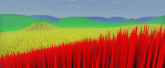
In the animated figure in 2.5 I have highlighted the different LOD levels. We can see that there are many red and yellow grass blades. By tweaking the LOD calculation we might turn some of the red grass blades into yellow grass blades and some more yellow grass blades into green grass blades this further reducing the number of triangles.
5 The Code#
You can find the full source code on my Github page. The post below will take you straight to the page of the respository.
My implementation of Eddie Lee’s real-time grass demo
By now you should be able to implement your own real-time grass renderer. Please let me know your thoughts and feel free to ask questions.